


Players
This paper divides the process of realizing the value of highway data assets into three key stages: original data collection, data processing, and data product development. Based on this process, the main stakeholders in distributing revenues from highway data assets can be divided into three roles: First, the original data collectors, namely the initial holders of road data, who complete the original collection of road data and own these data; second, the data processors, who add value to the original data through cleansing, integration, analysis, mining, and other means; third, the data product producers, who utilize the processed data for product design, development, and operation, realizing the full commercial value of the data assets.
Original data collectors
They obtain revenues by collecting road original data, which are primarily generated from enterprises’ activities in road construction and operation management. For example, traffic volume and speed data collected by road authorities through fixed monitoring devices; toll station traffic volume and toll data acquired by toll road operators; real-time traffic conditions and route data collected by map service companies using navigation devices; vehicle status and road condition data gathered by automakers through onboard devices.
Data processors
They obtain revenues by processing the lawfully acquired original road data using methods like standardization, cleansing, integration, mining, etc. This process requires building road data warehouses, establishing analytical models, and discovering correlations in the data to extract value from the data. Since the original road data has a large volume but low-value density, it cannot be directly used for knowledge discovery and decision support. Only by improving data quality and discovering potential value through processing can more valuable highway data assets formed. For example, road research institutes analyze and integrate data collected by road authorities to support transportation planning; intelligent connected vehicle companies develop data models, leveraging data gathered by onboard devices to forecast traffic volume; mobility service platforms fuse user feedback with driving data to enhance traffic condition judgment and vehicle dispatching capabilities.
Data product producers
Based on the processed datasets, they obtain revenues by developing data products with practical value, marketing, and maintaining these products. Major data product formats include data packages, API interfaces, data analytical reports, etc. These road data products require continuous development and maintenance by data product operators. For example, road monitoring systems developed by transportation authorities for government users to improve road safety; ETC systems developed by new infrastructure operators, providing services like toll payment inquiries; usage-based auto insurance products developed by insurance companies using vehicle driving data to charge premiums based on mileage.
It should be emphasized that since road data rights can be separated and shared, different interests can be allocated to different stakeholders as needed, and the same participant may also simultaneously take on roles in multiple stages of the data value chain. For example, some transportation operators are responsible for both original data collection and participation in data processing and product design. Therefore, the distribution of revenues from road data assets should be reasonably determined based on the contributions made by each participant at different stages.
Evaluation indicator system for revenue allocation
The traditional Shapley value method only allocates revenues based on marginal contributions, while participants in the same role may have significant differences in costs, risks, and other aspects. These differences need to be fully considered in the revenue distribution process. In addition, generating road data assets requires the participation of original data collectors, data processors, and data product producers. In practice, some participants may simultaneously take on multiple roles. The revenue distribution needs to comprehensively consider their contributions across different roles.
To address these issues, this paper proposes a two-layer allocation mechanism based on the traditional Shapley value method to reasonably distribute revenues from road data assets. The first layer determines the revenue shares for the three roles based on their contributions in the value chain; the second layer further distributes the revenues of each role to the actual participants. Compared to the Shapley value method, which only considers marginal contributions, this two-layer allocation mechanism is more comprehensive and reasonable, as it additionally takes into full consideration the differences in costs and risk sharing among different participants, as well as the contributions of the same participant under different roles. By considering both role contributions and participant efforts, the two-layer allocation mechanism achieves fair and effective revenue distribution.
First layer: role revenue allocation
During the lifecycle of road data assets, all participants face various risks, and those taking on more risks expect higher returns. Therefore, this paper takes the data risk factor as a correction factor for role benefit allocation. According to the sources, data risks are divided into external risks and internal risks. External risks mainly include policy risks and legal risks, as changes in relevant policies and the enactment of laws regarding data assets can significantly impact participants’ operations. Internal risks refer to those arising from equipment failures, data security, and other factors during the generation of road data assets, which can be prevented and controlled.
Second layer: revenue allocation among participants of the same role
Based on the characteristics of the three rolesâoriginal data collectors, data processors, and data product producersâspecific indicators that influence revenue distribution among participants within each role are constructed respectively.
For original data collectors, their contribution lies in planning the collection of high-value original data. This paper employs three indicatorsâconstruction cost, data demand, and data characteristicsâto adjust the revenue of the original data collection participants. Construction cost covers the major costs involved in the production process of original data, including sub-indicators of data planning, data collection, and data storage. Data demand is assessed by examining the scarcity and application value of the data in the market and is further divided into two sub-indicators: demand extent and scarcity level. Considering the large volume but low-value density of original road data, data coverage and timeliness of updates are included as sub-indicators under data characteristics.
For the data processors, their contribution lies in transforming the original data into high-quality data with application value. Two indicatorsâdata cleansing and data analysisâcan be adopted to evaluate the contribution of data processing participants. Data cleansing is considered the fundamental task in data processing, and its effectiveness can be assessed using the sub-indicators of data volume and data quality. As the core of extracting data value, data analysis can be evaluated based on the quality of analysis methods and analysis utility as sub-indicators.
For the data product producers, their contribution lies in developing products and services for end users based on processed data, as well as managing the operation of the products. Two indicatorsâproduct development and product maintenanceâcan be employed to assess the contribution of data product producers. Product development is evaluated based on the workload and difficulty coefficient as sub-indicators, while product maintenance is evaluated based on stability and update frequency as sub-indicators.
Overall, the evaluation indicator system for road data asset revenue allocation constructed in this paper comprehensively considers the contributions of different roles and participants in the road data asset value chain. The specific indicators are illustrated in Fig. 1, and Table 2 provides detailed explanations of the definitions, calculation methods, and value ranges for each indicator.
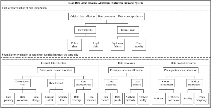
Evaluation indicator system for road data asset revenue allocation.
Conventional Shapley value
The Shapley value method is a cooperative game approach used to solve the problem of profit distribution in multi-party cooperation. It determines the allocation of profits for each participant based on their marginal contributions. It is known for its characteristics of simple model construction, easy solvability, and unique solutions, allowing for a balance between efficiency and fairness in the distribution process.
First layer: role revenue allocation
Suppose in a road data asset revenue distribution, the three roles of original data collectors, data processors, and data product producers are represented by the set \(R = \{ 1,2,3\}\). For any subset (representing any combination of roles in the role set), there exists a real-valued function \(v(s)\), satisfying:
$$v(s_{1} \cup s_{2} ) \ge v(s_{1} ) + v(s_{2} ),\begin{array}{*{20}c} {} & {s_{1} \cap s_{2} } \\ \end{array} = \emptyset ,\begin{array}{*{20}c} {} & {s_{1} ,s_{2} \subset R} \\ \end{array}$$
(1)
\([R,v]\) is termed the cooperation strategy of the three roles, and \(v\) represents the characteristic function of the cooperation strategy.
\(x_{i}\) denotes the fraction of the maximum revenue \(v(R)\) from the road data asset that role \(i\) receives. Based on the cooperative strategies \([R,v]\), the income distribution among the three roles is represented by \(x = (x_{1} ,x_{2} ,x_{3} )\). A successful cooperative strategy must satisfy the following conditions:
$$\begin{array}{*{20}c} {x_{1} + x_{2} + x_{3} = v(R)} & {i = 1,2,3} \\ \end{array}$$
$$x_{i} \ge v(i),\begin{array}{*{20}c} {} & {i = 1,2,3} \\ \end{array}$$
(2)
where \(\varphi_{i} (v)\) represents the distribution obtained by role \(i\) under the cooperative strategy \([R,v]\). The Shapley value for each role’s income distribution under the cooperative strategies is given by \(\Phi (v) = (\varphi_{1} (v),\varphi_{2} (v),\varphi_{3} (v))\):
$$\varphi_{i} (v) = \sum\limits_{{s \in s_{i} }} {w(\left| s \right|)[v(s) – v(s\backslash i)]\begin{array}{*{20}c} {} & {i = 1,2,3} \\ \end{array} }$$
$$w(\left| s \right|) = \frac{(3 – \left| s \right|)!(\left| s \right| – 1)!}{{3!}}$$
$$\varphi_{1} (v) + \varphi_{2} (v) + \varphi_{3} (v) = v(R)$$
(3)
where \(s_{i}\) is a set containing all subsets of \(R\) that include role \(i\), \(\left| s \right|\) is the number of elements in subset \(s\), \(w(\left| s \right|)\) is the weighting factor, \(v(s)\) is the revenue for subset \(s\), and \(v(s\backslash i)\) represents the revenue that can be obtained by removing role \(i\) from subset \(s\).
Therefore, the Shapley value method is applied to evaluate the contributions of the three roles in the road data asset, and the calculations for revenue allocation are presented in Table 3.
Second layer: revenue allocation among participants of the same role
Once the Shapley values \(\Phi (v) = (\varphi_{1} (v),\varphi_{2} (v),\varphi_{3} (v))\) for revenue allocation among the three roles in a road data asset are determined, it is necessary to determine the specific distribution of benefits to the participants under the same role based on the \(\varphi_{i} (v)\) values of each role, to realize the distribution of benefits from the road data asset to each participant.
Assuming that there are \(n\) participants in a road data asset revenue allocation, the number of participants with the roles of original data collectors, data processors, and data product producers is \(n_{i}\)(\(i = 1,2,3\)), and it is clear that \(n_{1} + n_{2} + n_{3} \ge n\). Denote \(\varphi_{{_{j} }}^{i} (v)\) as the profit obtained by \(j{\text{ th}}\) participant when distributing the profit \(\varphi_{i} (v)\) of role \(i\):
$$\varphi_{{_{j} }}^{i} (v) = \sum\limits_{{s \in s_{j}^{i} }} {w(\left| s \right|)[v(s) – v(s\backslash j)]\begin{array}{*{20}c} {} & {j = 1,2, \ldots ,n_{i} } \\ \end{array} }$$
$$w(\left| s \right|) = \frac{{(n_{i} – \left| s \right|)!(\left| s \right| – 1)!}}{{n_{i} !}}$$
$$\sum\limits_{j = 1}^{{n_{i} }} {\varphi_{j}^{i} } (v) = \varphi_{i} (v)\begin{array}{*{20}c} {} & {i = 1,2,3} \\ \end{array}$$
(4)
where \(s_{{_{j} }}^{i}\) represents the set of all subsets of participants within role \(i\) that includes participant \(j\), \(\left| s \right|\) is the number of elements in subset \(s\), \(w(\left| s \right|)\) is the weighting factor, \(v(s)\) is the profit for subset \(s\), and \(v(s\backslash j)\) denotes the profit that can be obtained by excluding participant \(j\) from subset \(s\).
Synthesis of revenue allocation among participants
After calculating the revenue distribution for each participant within each role, it is necessary to synthesize the revenue distribution among participants under different roles, taking into account their contributions at different stages.
Let \(N = \{ 1,2, \ldots ,n\}\) be the set of participants, and \(N_{i} = \{ 1,2, \ldots ,n_{i} \}\)(\(i = 1,2,3\)) represents the set of participants for the roles of original data collectors, data processors, and data product producers, respectively. Clearly \(N_{i} \subset N\), due to the different sizes and order of elements in sets \(N\) and \(N_{i}\), we define a function \(f_{i} :N \to N_{i}\) that, for each element \(x\)(\(x = 1,2, \ldots n\)) in set \(N\), maps it to the corresponding element in set \(N_{i}\), if there exists an element \(j \in N_{i}\) such that \(f_{i} (x) = j\), otherwise there is no corresponding element in set \(N_{i}\). Therefore, the profit distribution for each participant \(x\) in different roles \(i\) can be represented as \(\hat{\varphi }_{{_{x} }}^{i} (v)\), where:
$$\hat{\varphi }_{{_{x} }}^{i} (v) = \left\{ {\begin{array}{*{20}r} \hfill {\varphi_{{_{j} }}^{i} (v),\begin{array}{*{20}c} {} & {if} \\ \end{array} \begin{array}{*{20}c} {} & {f_{i} (x) = j} \\ \end{array} } \\ \hfill {0,\begin{array}{*{20}c} {} & {} & {if\begin{array}{*{20}c} {} & {f_{i} (x) \ne j} \\ \end{array} } \\ \end{array} } \\ \end{array} } \right.\begin{array}{*{20}c} {} & {i = 1,2,3} \\ \end{array}$$
(5)
To synthesize the profit values for each participant in different roles, we obtain the total profit distribution \(\overline{\varphi }_{x} (v)\) for the participant in the road data asset, denoted as:
$$\overline{\varphi }_{x} (v) = \hat{\varphi }_{{_{x} }}^{1} (v) + \hat{\varphi }_{{_{x} }}^{2} (v) + \hat{\varphi }_{{_{x} }}^{3} (v)$$
(6)
The modified Shapley value
The traditional Shapley value method only determines revenue allocation based on marginal contributions, without considering differences among participants in terms of costs and risks. To achieve fair profit distribution of road data assets, it is essential to comprehensively evaluate the differences among roles and participants in terms of input costs, risk allocation, and other aspects. In this paper, based on the traditional Shapley value method, a revenue allocation evaluation indicator system for the road data asset, as depicted in Fig. 1, is established. This indicator-driven two-layer allocation correction scheme is used to modify the revenue allocation among different roles and participants. By doing so, a more equitable and reasonable revenue allocation model for the road data asset is developed. The architecture of the improved revenue allocation model for the road data asset is illustrated in Fig. 2.
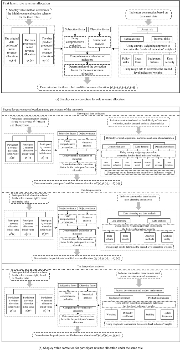
Architecture of the improved revenue allocation model for road data assets.
Calculation of weights for evaluating revenue allocation of road data assets
Calculation of primary indicator weight
This study utilizes the entropy weighting method to calculate the weights of primary evaluation indicators in Fig. 1. It is assumed that \(m\) expert will be invited to evaluate the importance of \(I\) primary indicators and obtain a scoring matrix \(S = (s_{ij} )_{m \times I}\), \(i = 1,2, \ldots ,m\), \(j = 1,2, \ldots ,I\), where \(s_{ij}\) represents the rating provided by the \(i\) expert for the \(j\) indicator.
If \(j\) denotes a profit-related indicator, normalization is performed according to Eq. (7):
$$\hat{s}_{ij} = \frac{{s_{ij} – \mathop {\min }\limits_{i} \{ s_{ij} \} }}{{\mathop {\max }\limits_{i} \{ s_{ij} \} – \mathop {\min }\limits_{i} \{ s_{ij} \} }}$$
(7)
If \(j\) denotes a cost-related indicator, normalization is performed according to Eq. (8):
$$\hat{s}_{ij} = \frac{{\mathop {\max }\limits_{i} \{ s_{ij} \} – s_{ij} }}{{\mathop {\max }\limits_{i} \{ s_{ij} \} – \mathop {\min }\limits_{i} \{ s_{ij} \} }}$$
(8)
The weights \(p_{ij}\) of the scores given by different experts to each indicator are calculated using the entropy weighting method, as shown in Eq. (9):
$$p_{ij} = \frac{{\hat{s}_{ij} }}{{\sum\limits_{i = 1}^{m} {\hat{s}_{ij} } }}$$
(9)
The information entropy value \(e_{j}\) is calculated separately for each indicator \(j\) according to \(p_{ij}\):
$$e_{j} = – \frac{1}{\ln m}\sum\limits_{i = 1}^{m} {p_{ij} \ln p_{ij} }$$
(10)
To ensure that the entropy value \(e_{j}\) holds numerical significance, we set \(\ln p_{ij} = 0\) when \(p_{ij} = 0\).
The entropy weight \(\omega_{j}\) for each indicator is then calculated based on the entropy value \(e_{j}\), as follows:
$$\omega_{j} = \frac{{1 – e_{j} }}{{\sum\limits_{j = 1}^{I} {(1 – e_{j} )} }}$$
(11)
Calculation of secondary indicator weight
For the secondary evaluation indicators in Fig. 1, the rough set theory is employed in this study to calculate their indicator weights. It is assumed that \(m\) experts are invited to assess the importance of \(I_{j}\) secondary indicators under the \(j\)(\(j = 1,2, \ldots ,I\)) primary indicator, leading to the construction of an evaluation information system \(S_{j} = (U,A_{j} ,V_{j} ,f)\), where: the universe of discourse \(U = \{ 1,2, \ldots ,m\}\), a non-empty finite attribute set \(A_{j} = \{ a_{1} ,a_{2} , \ldots ,a_{{I_{j} }} \}\), and the attribute value domain \(V_{j}\) are obtained through expert assessment using a percentage-based scoring system. Moreover, \(f\) represents the relationship set between \(U\) and \(A_{j}\), also referred to as the information function set.
Definition 1
Let \(R\) be an equivalence relation on \(U\), denoted as:
$$ind(R) = \{ (x,y) \in U \times U|\forall a \in A_{j} ,f(x,a) = f(y,a)\}$$
(12)
\(U/ind(R)\) is referred to as the partition of \(U\), and each element \(a\) is called an equivalence class.
In an information system \(S_{j}\), different attributes have varying effects, and some attributes may even be redundant. Therefore, it is necessary to eliminate irrelevant or unimportant knowledge from the information system while maintaining its classification ability. This process is known as knowledge reduction. Knowledge reduction is divided into attribute reduction and attribute value reduction. However, since attribute value reduction is relatively straightforward, knowledge reduction generally refers to attribute reduction in most cases.
Definition 2
If \(ind(R) = ind(R – \{ r\} )\), it is referred to \(r\) as reducible knowledge in the information system \(R\). If \(P = R – \{ r\}\) is independent, then \(P\) is a knowledge reduction in \(R\).
In the information system \(S_{j}\), the set of secondary indicators for the primary indicator \(j\) is denoted as \(A_{j} = \{ a_{1} ,a_{2} , \ldots ,a_{{I_{j} }} \}\). Assume that there are \(l_{j}\) sets of \(A_{j}\) divisions over \(U\), represented as \(U/ind(A) = \{ X_{1} ,X_{2} , \ldots ,X_{{l_{j} }} \}\). The information quantity of \(A_{j}\) is calculated as:
$$I(A_{j} ) = \sum\limits_{i = 1}^{{l_{j} }} {\frac{{\left| {X_{i} } \right|}}{\left| U \right|}\left[ {1 – \frac{{\left| {X_{i} } \right|}}{\left| U \right|}} \right]} = 1 – \frac{1}{{\left| U \right|^{2} }}\sum\limits_{i = 1}^{{l_{j} }} {\left| {X_{i} } \right|^{2} }$$
(13)
where \(\left| U \right|\) represents the number of elements in the universe of discourse \(U\), and \(\left| {X_{i} } \right|\) denotes the number of elements in the \(i{\text{ th}}\) set.
In the information system \(S_{j}\), for the knowledge reduction \(ind(A_{j} – \{ a\} )\) of \(\forall a \in A_{j}\), let there exist \(l_{a}\) sets of the partition of \(U\) after reduction, denoted as \(U/ind(A_{j} – \{ a\} ) = \{ X_{1} ,X_{2} , \ldots ,X_{{l_{a} }} \}\). The information quantity of \(A_{j} – \{ a\}\) is given by:
$$I(A_{j} – \{ a\} ) = \sum\limits_{i = 1}^{{l_{a} }} {\frac{{\left| {X_{i} } \right|}}{\left| U \right|}\left[ {1 – \frac{{\left| {X_{i} } \right|}}{\left| U \right|}} \right]} = 1 – \frac{1}{{\left| U \right|^{2} }}\sum\limits_{i = 1}^{{l_{a} }} {\left| {X_{i} } \right|^{2} }$$
(14)
Therefore, the importance of \(a\) in \(A_{j}\) can be expressed as:
$$Sig_{{A_{j} }} (a) = I(A_{j} ) – I(A_{j} – \{ a\} )$$
(15)
The weights of secondary indicators \(A_{j} = \{ a_{1} ,a_{2} , \ldots ,a_{{I_{j} }} \}\) under the primary indicator \(j\) can be calculated based on their importance using the equation:
$$\omega_{{A_{j} }} (a) = \frac{{Sig_{{A_{j} }} (a)}}{{\sum\limits_{a = 1}^{{I_{j} }} {Sig_{{A_{j} }} (a)} }}$$
(16)
By incorporating the entropy weight \(\omega_{j}\) of the primary indicator \(j\), the final weights of the secondary indicators \(A_{j} = \{ a_{1} ,a_{2} , \ldots ,a_{{I_{j} }} \}\) can be determined as:
$$\tilde{\omega }_{{A_{j} }} (a) = \omega_{j} \times \omega_{{A_{j} }} (a),\;\;\;\;\;a = 1,2, \cdots I_{j} ,j = 1,2, \ldots ,I$$
(17)
Evaluation of revenue allocation indicators for road data assets
Once the weights of the revenue allocation evaluation indicators for road data assets are determined, it is necessary to numerically evaluate different schemes under the relevant indicators. As some indicators involve subjective measures and others are objective numerical metrics, different methods are required to quantify both subjective and objective factors for an effective assessment of revenue allocation indicators for road data assets.
Defining a scheme as a collective term for subjects involved in revenue allocation across different layers, the scheme represents roles at the first layer and participants within each role at the second layer. Assuming that there are \(D\) schemes involved in the distribution of a road data asset, scheme \(d\)(\(d = 1,2, \ldots ,D\)), requires a comprehensive evaluation of all secondary indicators under \(I\) primary indicators. Let there be \(I_{j}\) secondary indicators under the \(j{\text{ th}}\)(\(j = 1,2, \ldots ,I\)) primary indicator, and the set of indicators is \(A_{j} = \{ a_{1} ,a_{2} , \ldots ,a_{{I_{j} }} \}\), of which there are \(\dot{I}_{j}\) subjective indicators and \(\ddot{I}_{j}\) objective indicators, and \(\dot{I}_{j} + \ddot{I}_{j} = I_{j}\), let the set of subjective secondary indicators under the \(j{\text{ th}}\) primary indicator be \(A^{\prime}_{j} = \{ a^{\prime}_{1} ,a^{\prime}_{2} , \ldots ,a^{\prime}_{{\dot{I}_{j} }} \}\), \(a^{\prime}_{i} \in A_{j} ,i = 1,2, \ldots ,\dot{I}_{j}\), and the set of objective secondary indicators be \(A^{\prime\prime}_{j} = \{ a^{\prime\prime}_{1} ,a^{\prime\prime}_{2} , \ldots ,a^{\prime\prime}_{{\ddot{I}_{j} }} \}\), \(a^{\prime\prime}_{i} \in A_{j} ,i = 1,2, \ldots ,\ddot{I}_{j}\), and \(A^{\prime}_{j} \cup A^{\prime\prime}_{j} = A_{j}\), \(A^{\prime}_{j} \cap A^{\prime\prime}_{j} = \emptyset\).
Subjective evaluation
Suppose \(m\) experts are invited to assess scheme \(d\) based on the subjective indicator set \(A^{\prime}_{j} = \{ a^{\prime}_{1} ,a^{\prime}_{2} , \ldots ,a^{\prime}_{{\dot{I}_{j} }} \}\) for indicator \(j\). Based on the comment set \(V =\){low, moderately low, moderate, moderately high, high}, a fuzzy evaluation is conducted to obtain the fuzzy relationship matrix:
$$R_{j} (d) = \left[ {\begin{array}{*{20}c} {r_{{a^{\prime}_{1} }}^{1} (d)} & {r_{{a^{\prime}_{1} }}^{2} (d)} & {r_{{a^{\prime}_{1} }}^{3} (d)} & {r_{{a^{\prime}_{1} }}^{4} (d)} & {r_{{a^{\prime}_{1} }}^{5} (d)} \\ {r_{{a^{\prime}_{2} }}^{1} (d)} & {r_{{a^{\prime}_{2} }}^{2} (d)} & {r_{{a^{\prime}_{2} }}^{3} (d)} & {r_{{a^{\prime}_{2} }}^{4} (d)} & {r_{{a^{\prime}_{2} }}^{5} (d)} \\ \vdots & \vdots & \vdots & \vdots & \vdots \\ {r_{{a^{\prime}_{{\dot{I}_{j} }} }}^{1} (d)} & {r_{{a^{\prime}_{{\dot{I}_{j} }} }}^{2} (d)} & {r_{{a^{\prime}_{{\dot{I}_{j} }} }}^{3} (d)} & {r_{{a^{\prime}_{{\dot{I}_{j} }} }}^{4} (d)} & {r_{{a^{\prime}_{{\dot{I}_{j} }} }}^{5} (d)} \\ \end{array} } \right]$$
(18)
Among them, \(r_{{a^{\prime}_{i} }}^{1} (d)\), \(r_{{a^{\prime}_{i} }}^{2} (d)\), \(r_{{a^{\prime}_{i} }}^{3} (d)\), \(r_{{a^{\prime}_{i} }}^{4} (d)\), and \(r_{{a^{\prime}_{i} }}^{5} (d)\) respectively represent the frequency distribution of indicator \(a^{\prime}_{i}\)(\(i = 1,2, \ldots ,\dot{I}_{j}\)) under the five comments of low, moderately low, moderate, moderately high, and high.
Based on the indicator weights calculated according to Eq. (17), the subjective indicator weight vector for Indicator \(A^{\prime}_{j}\) is denoted as \(\tilde{\omega }_{{A^{\prime}_{j} }} = [\tilde{\omega }_{{A^{\prime}_{j} }} (a^{\prime}_{1} ),\tilde{\omega }_{{A^{\prime}_{j} }} (a^{\prime}_{2} ), \ldots ,\tilde{\omega }_{{A^{\prime}_{j} }} (a^{\prime}_{{\dot{I}_{j} }} )]\). Using this weight vector, the fuzzy evaluation vector is obtained as:
$$T_{j} (d) = \tilde{\omega }_{{A^{\prime}_{j} }} \times R_{j} (d)$$
(19)
where \(T_{j} (d)\) is referred to as the fuzzy evaluation vector.
Using the membership degree of the comment set \(V =\){low, moderately low, moderate, moderately high, high}, the membership degree vector \(\overline{V} = [0.1,0.3,0.5,0.7,0.9]\) can be determined. From this, the evaluation value \(L^{\prime}_{j} (d)\) of the subjective component for indicator \(j\) can be calculated as:
$$L^{\prime}_{j} (d) = T_{j} (d) \times \overline{V}^{T}$$
(20)
The subjective evaluation values for \(I\) primary indicators are synthesized as:
$$L^{\prime}(d) = \sum\limits_{j = 1}^{I} {L^{\prime}_{j} (d)}$$
(21)
where \(L^{\prime}(d)\) is termed as the subjective evaluation value of scheme \(d\).
Objective evaluation
In the set of objective indicators \(A^{\prime\prime}_{j} = \{ a^{\prime\prime}_{1} ,a^{\prime\prime}_{2} , \ldots ,a^{\prime\prime}_{{\ddot{I}_{j} }} \}\), the numerical value for each indicator of Scheme \(d\) is represented by a vector, denoted as \(f_{d} (A^{\prime\prime}_{j} ) = [f_{d} (a^{\prime\prime}_{1} ),f_{d} (a^{\prime\prime}_{2} ), \ldots ,f_{d} (a^{\prime\prime}_{{\ddot{I}_{j} }} )]\). For the indicator \(a^{\prime\prime}_{i}\)(\(i = 1,2, \ldots ,\ddot{I}_{j}\)), if it is a revenue indicator, it is normalized on the scheme \(D\) according to Eq. (22), and if it is a cost indicator, the values are normalized using Eq. (23). This normalization process yields the normalized value vector, denoted as \(\tilde{f}_{d} (A^{\prime\prime}_{j} ) = [\tilde{f}_{d} (a^{\prime\prime}_{1} ),\tilde{f}_{d} (a^{\prime\prime}_{2} ), \ldots ,\tilde{f}_{d} (a^{\prime\prime}_{{\ddot{I}_{j} }} )]\), where it is evident that \(\sum\limits_{d = 1}^{D} {\tilde{f}_{d} (a^{\prime\prime}_{i} } ) = 1\).
$$\tilde{f}_{d} (a^{\prime\prime}_{i} ) = \frac{{f_{d} (a^{\prime\prime}_{i} )}}{{\sum\limits_{d = 1}^{D} {f_{d} (a^{\prime\prime}_{i} } )}}$$
(22)
$$\tilde{f}_{d} (a^{\prime\prime}_{i} ) = 1 – \frac{{f_{d} (a^{\prime\prime}_{i} )}}{{\sum\limits_{d = 1}^{D} {f_{d} (a^{\prime\prime}_{i} } )}}$$
(23)
According to the weights of the indicators calculated in Eq. (17), the weight vector \(\tilde{\omega }_{{A^{\prime\prime}_{j} }} = [\tilde{\omega }_{{A^{\prime\prime}_{j} }} (a^{\prime\prime}_{1} ),\tilde{\omega }_{{A^{\prime\prime}_{j} }} (a^{\prime\prime}_{2} ), \ldots ,\tilde{\omega }_{{A^{\prime\prime}_{j} }} (a^{\prime\prime}_{{\ddot{I}_{j} }} )]\) of the objective indicator \(A^{\prime\prime}_{j}\) can be obtained, and based on the vector of normalized values \(\tilde{f}_{d} (A^{\prime\prime}_{j} )\), the evaluation value of the objective part of the indicator \(j\) is calculated as \(L^{\prime\prime}_{j} (d)\):
$$L^{\prime\prime}_{j} (d) = \tilde{\omega }_{{A^{\prime\prime}_{j} }} \times \tilde{f}_{d} (A^{\prime\prime}_{j} )^{T}$$
(24)
Synthesize the assessed value of the objective component of the \(I\) primary indicators indicator:
$$L^{\prime\prime}(d) = \sum\limits_{j = 1}^{I} {L^{\prime\prime}_{j} (d)}$$
(25)
where \(L^{\prime\prime}(d)\) is called the objective evaluation value of scheme \(d\).
Integration of objective and subjective evaluations
Combine the subjective and objective evaluation values for scheme \(d\) to obtain the composite evaluation value.
$$L(d) = \alpha L^{\prime}(d) + (1 – \alpha )L^{\prime\prime}(d),d = 1,2, \ldots ,D$$
(26)
where \(L(d)\) is the composite evaluated value of scheme \(d\) and \(\alpha\)(\(0 \le \alpha \le 1\)) is the weighting factor, allowing for the adjustment of the importance of subjective and objective evaluation values in the composite evaluated value.
Normalize the composite evaluated value \(L(d)\) of scheme \(d\):
$$\tilde{L}(d) = \frac{L(d)}{{\sum\limits_{d = 1}^{D} {L(d)} }},d = 1,2, \ldots ,D$$
(27)
The modification of road data asset revenue allocation
Role revenue allocation modification
Based on Eq. (3), the initial allocations for the roles \(R = \{ 1,2,3\}\) of the original data collectors, data processors, and data product producers can be computed, denoted as \(\Phi (v) = (\varphi_{1} (v),\varphi_{2} (v),\varphi_{3} (v))\). Additionally, it is known that \(\varphi_{1} (v) + \varphi_{2} (v) + \varphi_{3} (v) = v(R)\), where \(v(R)\) represents the maximum revenue for the road data asset.
As illustrated in Fig. 2a, based on the model in Section “Evaluation of revenue allocation indicators for road data assets”, the comprehensive evaluation values \(\tilde{L}_{R} (1)\), \(\tilde{L}_{R} (2)\), and \(\tilde{L}_{R} (3)\) for the roles of the original data collectors, data processors, and data product producers can be calculated.
Next, compute the role revenue allocation modification factor:
$$\Delta \theta_{i} = \tilde{L}_{R} (i) – \frac{1}{3},i = 1,2,3$$
(28)
The modified value of the role’s revenue allocation is:
$$\tilde{\varphi }_{i} (v) = \varphi_{i} (v) + \Delta \theta_{i} \times v(R),i = 1,2,3$$
(29)
Participant revenue allocation modification within the same role
Suppose there are \(n\) participants involved in the distribution of road data asset profits, and the number of participants in the roles of data collectors, data processors, and data product producers is denoted as \(n_{i}\)(\(i = 1,2,3\)). According to Eq. (4), we determine the initial distribution scheme \(\Phi^{i} (v) = (\varphi_{{_{1} }}^{i} (v),\varphi_{{_{2} }}^{i} (v), \ldots ,\varphi_{{_{{n_{i} }} }}^{i} (v))\) of participants within the role \(i\) based on the role revenue allocation modified value \(\tilde{\varphi }_{i} (v)\), where \(\sum\limits_{j = 1}^{{n_{i} }} {\varphi_{j}^{i} (v)} = \tilde{\varphi }_{i} (v),i = 1,2,3\).
As shown in Fig. 2b, applying the model in Section “Evaluation of revenue allocation indicators for road data assets”, we can calculate the comprehensive evaluation value \([\tilde{L}^{1} (1),\tilde{L}^{1} (2), \ldots ,\tilde{L}^{1} (n_{1} )]\) for participants within the data collectors.
To modify the revenue allocation for participants within the data collectors, we compute the participant modification factor as follows:
$$\Delta \theta_{j}^{1} = \tilde{L}^{1} (j) – \frac{1}{{n_{1} }},j = 1,2, \ldots ,n_{1}$$
(30)
The modified values for participant revenue allocation within the data collectors are then given by:
$$\tilde{\varphi }_{j}^{1} (v) = \varphi_{j}^{1} (v) + \Delta \theta_{j}^{1} \times \tilde{\varphi }_{1} (v)$$
(31)
Similarly, using the model in Section “Evaluation of revenue allocation indicators for road data assets”, we can calculate the comprehensive evaluation value \([\tilde{L}^{2} (1),\tilde{L}^{2} (2), \ldots ,\tilde{L}^{2} (n_{2} )]\) for participants within the data processors.
For the data processors, the participant revenue allocation modification factor is calculated as follows:
$$\Delta \theta_{j}^{2} = \tilde{L}^{2} (j) – \frac{1}{{n_{2} }},j = 1,2, \ldots ,n_{2}$$
(32)
The modified values for participant revenue allocation within the data processors are then obtained as:
$$\tilde{\varphi }_{j}^{2} (v) = \varphi_{j}^{2} (v) + \Delta \theta_{j}^{2} \times \tilde{\varphi }_{2} (v)$$
(33)
Likewise, considering the model in Section “Evaluation of revenue allocation indicators for road data assets”, we can compute the comprehensive evaluation value \([\tilde{L}^{3} (1),\tilde{L}^{3} (2), \ldots ,\tilde{L}^{3} (n_{3} )]\) for participants within the data product producers.
To modify the revenue allocation for participants within the data product producers, we calculate the participant revenue allocation modification factor as follows:
$$\Delta \theta_{j}^{3} = \tilde{L}^{3} (j) – \frac{1}{{n_{3} }},j = 1,2, \ldots ,n_{3}$$
(34)
Finally, the modified values for participant revenue allocation within the data product producers are given by:
$$\tilde{\varphi }_{j}^{3} (v) = \varphi_{j}^{3} (v) + \Delta \theta_{j}^{3} \times \tilde{\varphi }_{3} (v)$$
(35)
Final revenue allocation scheme for participants
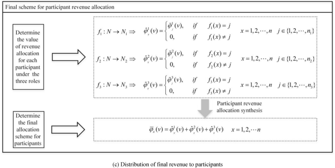
As depicted in Fig. 2(c), using Eq. (5), we determine the revenue allocation modified values for the \(n\) participants across the three roles:
$$\hat{\varphi }_{{_{x} }}^{i} (v) = \left\{ {\begin{array}{*{20}r} \hfill {\tilde{\varphi }_{{_{j} }}^{i} (v),\begin{array}{*{20}c} {} & {if} \\ \end{array} \begin{array}{*{20}c} {} & {f_{i} (x) = j} \\ \end{array} } \\ \hfill {0,\begin{array}{*{20}c} {} & {} & {if\begin{array}{*{20}c} {} & {f_{i} (x) \ne j} \\ \end{array} } \\ \end{array} } \\ \end{array} } \right.\begin{array}{*{20}c} {} & {x = 1,2, \ldots ,n;\begin{array}{*{20}c} {} \\ \end{array} i = 1,2,3} \\ \end{array}$$
(36)
By synthesizing the profit values for each participant across the different roles, we obtain the final revenue allocation values for each participant involved in the road data asset:
$$\overline{\varphi }_{x} (v) = \hat{\varphi }_{{_{x} }}^{1} (v) + \hat{\varphi }_{{_{x} }}^{2} (v) + \hat{\varphi }_{{_{x} }}^{3} (v)\begin{array}{*{20}c} {} & {x = 1,2, \ldots ,n} \\ \end{array}$$
(37)